How does Stable Diffusion work?

Stable Diffusion is a latent diffusion model that generates AI images from text. Instead of operating in the high-dimensional image space, it first compresses the image into the latent space.

We will dig deep into understanding how it works under the hood.

Why do you need to know? Apart from being a fascinating subject in its own right, some understanding of the inner mechanics will make you a better artist. You can use the tool correctly to achieve results with higher precision.

How does text-to-image differ from image-to-image? What’s the CFG scale? What’s denoising strength? You will find the answer in this article.

Let’s dive in.

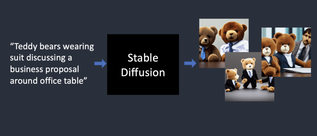
What can Stable Diffusion do?

In the simplest form, Stable Diffusion is a text-to-image model. Give it a text prompt. It will return an AI image matching the text.

Diffusion model

Stable Diffusion belongs to a class of deep learning models called diffusion models. They are generative models, meaning they are designed to generate new data similar to what they have seen in training. In the case of Stable Diffusion, the data are images.

Why is it called the diffusion model? Because its math looks very much like diffusion in physics. Let’s go through the idea.

Let’s say I trained a diffusion model with only two kinds of images: cats and dogs. In the figure below, the two peaks on the left represent the groups of cat and dog images.

Forward diffusion

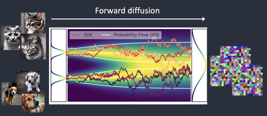
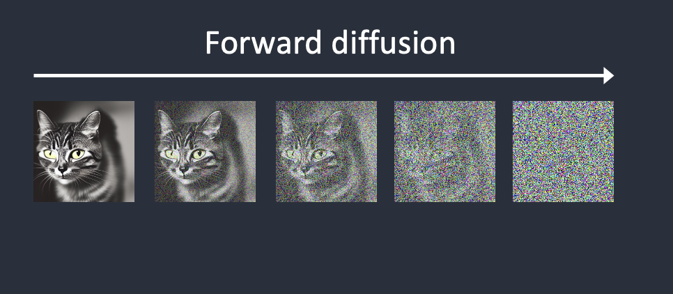
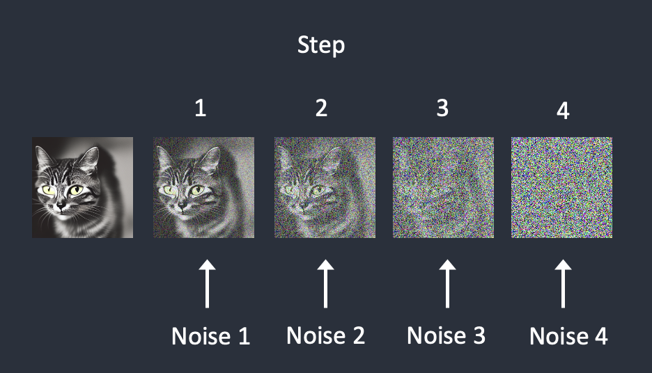
A forward diffusion process adds noise to a training image, gradually turning it into an uncharacteristic noise image. The forward process will turn any cat or dog image into a noise image. Eventually, you won’t be able to tell whether they are initially a dog or a cat. (This is important)

It’s like a drop of ink fell into a glass of water. The ink drop diffuses in water. After a few minutes, It randomly distributes itself throughout the water. You can no longer tell whether it initially fell at the center or near the rim.

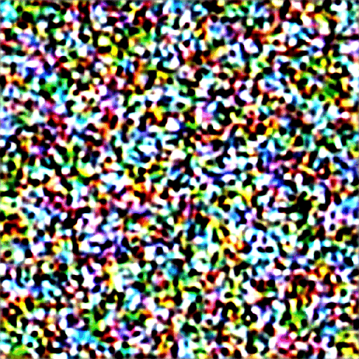
Below is an example of an image undergoing forward diffusion. The cat image turns to random noise.

Reverse diffusion

Now comes the exciting part. What if we can reverse the diffusion? Like playing a video backward. Going backward in time. We will see where the ink drop was initially added.

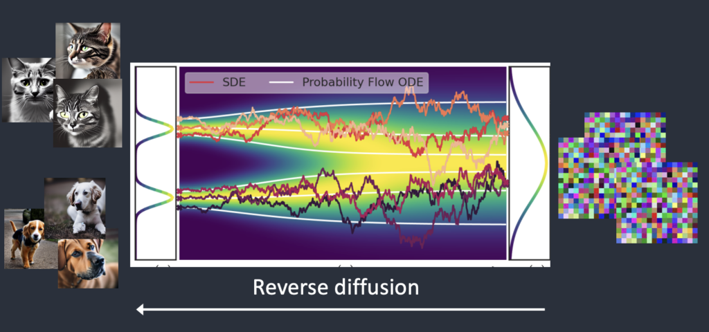
Starting from a noisy, meaningless image, reverse diffusion recovers a cat OR a dog image. This is the main idea.

Technically, every diffusion process has two parts: (1) drift and (2) random motion. The reverse diffusion drifts towards either cat OR dog images but nothing in between. That’s why the result can either be a cat or a dog.

How training is done

The idea of reverse diffusion is undoubtedly clever and elegant. But the million-dollar question is, “How can it be done?”

To reverse the diffusion, we need to know how much noise is added to an image. The answer is teaching a neural network model to predict the noise added. It is called the noise predictor in Stable Diffusion. It is a U-Net model. The training goes as follows.

1. Pick a training image, like a photo of a cat.
2. Generate a random noise image.
3. Corrupt the training image by adding this noisy image up to a certain number of steps.
4. Teach the noise predictor to tell us how much noise was added. This is done by tuning its weights and showing it the correct answer.

After training, we have a noise predictor capable of estimating the noise added to an image.

Reverse diffusion

Now we have the noise predictor. How to use it?

We first generate a completely random image and ask the noise predictor to tell us the noise. We then subtract this estimated noise from the original image. Repeat this process a few times. You will get an image of either a cat or a dog.

You may notice we have no control over generating a cat or dog’s image. We will address this when we talk about conditioning. For now, image generation is unconditioned.

You can read more about reverse diffusion sampling and samplers in this article.

Stable Diffusion model

Now I need to tell you some bad news: What we just talked about is NOT how Stable Diffusion works! The reason is that the above diffusion process is in image space. It is computationally very, very slow. You won’t be able to run on any single GPU, let alone the crappy GPU on your laptop.

The image space is enormous. Think about it: a 512×512 image with three color channels (red, green, and blue) is a 786,432-dimensional space! (You need to specify that many values for ONE image.)

Diffusion models like Google’s Imagen and Open AI’s DALL-E are in pixel space. They have used some tricks to make the model faster but still not enough.

Latent diffusion model

Stable Diffusion is designed to solve the speed problem. Here’s how.

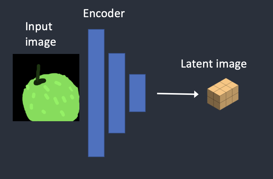
Stable Diffusion is a latent diffusion model. Instead of operating in the high-dimensional image space, it first compresses the image into the latent space. The latent space is 48 times smaller so it reaps the benefit of crunching a lot fewer numbers. That’s why it’s a lot faster.

Variational Autoencoder

It is done using a technique called the variational autoencoder. Yes, that’s precisely what the VAE files are, but I will make it crystal clear later.

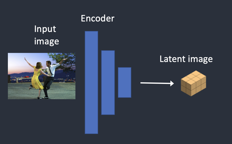
The Variational Autoencoder (VAE) neural network has two parts: (1) an encoder and (2) a decoder. The encoder compresses an image to a lower dimensional representation in the latent space. The decoder restores the image from the latent space.

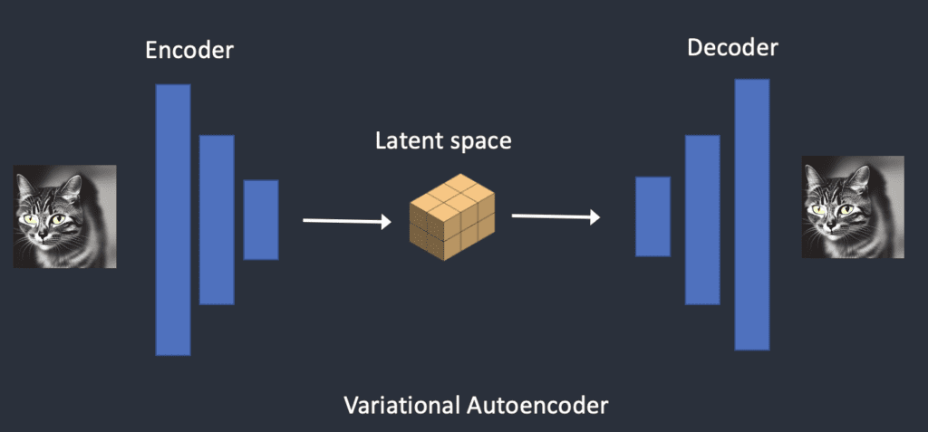
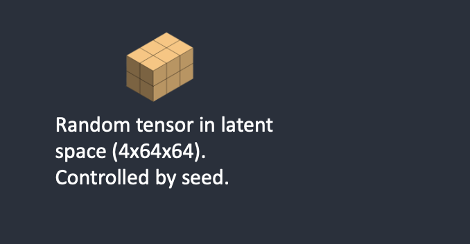
The latent space of Stable Diffusion model is 4x64x64, 48 times smaller than the image pixel space. All the forward and reverse diffusions we talked about are actually done in the latent space.

So during training, instead of generating a noisy image, it generates a random tensor in latent space (latent noise). Instead of corrupting an image with noise, it corrupts the representation of the image in latent space with the latent noise. The reason for doing that is it is a lot faster since the latent space is smaller.

Image resolution

The image resolution is reflected in the size of the latent image tensor. The size of the latent image is 4x64x64 for 512×512 images only. It is 4x96x64 for a 768×512 portrait image. That’s why it takes longer and more VRAM to generate a larger image.

Since Stable Diffusion v1 is fine-tuned on 512×512 images, generating images larger than 512×512 could result in duplicate objects, e.g., the infamous two heads.

Image upscaling

To generate a large print, keep at least one side of the image to 512 pixels. Use an AI upscaler or image-to-image function for image upscaling.

Alternatively, use the SDXL model. It has a larger default size of 1,024 x 1,024 pixels.

Why is latent space possible?

You may wonder why the VAE can compress an image into a much smaller latent space without losing information. The reason is, unsurprisingly, natural images are not random. They have high regularity: A face follows a specific spatial relationship between the eyes, nose, cheek, and mouth. A dog has 4 legs and is a particular shape.

In other words, the high dimensionality of images is artifactual. Natural images can be readily compressed into the much smaller latent space without losing any information. This is called the manifold hypothesis in machine learning.

Reverse diffusion in latent space

Here’s how latent reverse diffusion in Stable Diffusion works.

1. A random latent space matrix is generated.
2. The noise predictor estimates the noise of the latent matrix.
3. The estimated noise is then subtracted from the latent matrix.
4. Steps 2 and 3 are repeated up to specific sampling steps.
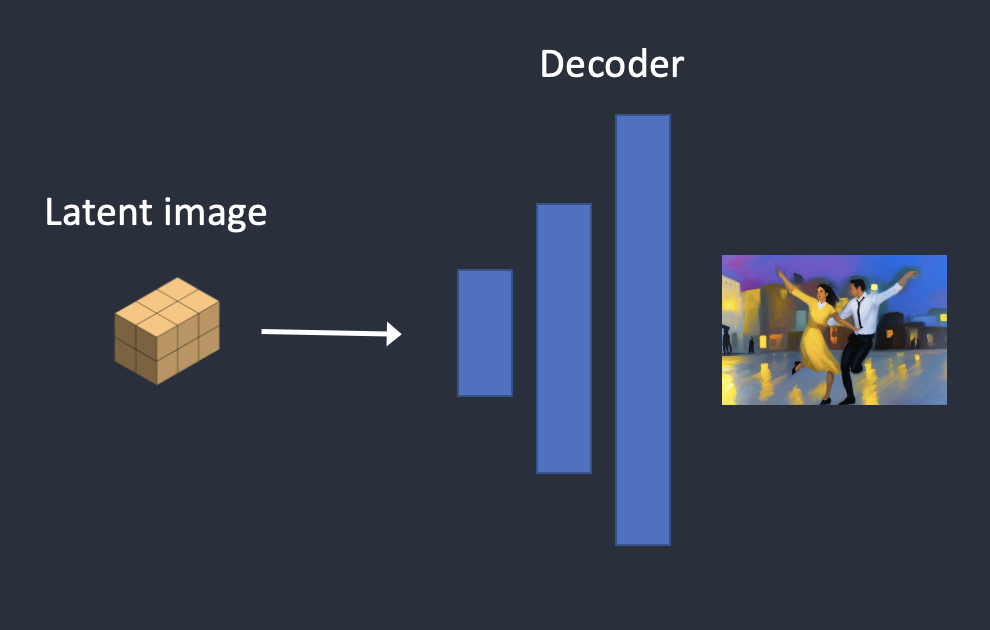
5. The decoder of VAE converts the latent matrix to the final image.

What is a VAE file?

VAE files are used in Stable Diffusion v1 to improve eyes and faces. They are the decoder of the autoencoder we just talked about. By further fine-tuning the decoder, the model can paint finer details.

You may realize what I have mentioned previously is not entirely true. Compressing an image into the latent space does lose information since the original VAE did not recover the fine details. Instead, the VAE decoder is responsible for painting fine details.

Conditioning

Our understanding is incomplete: Where does the text prompt enter the picture? Without it, Stable Diffusion is not a text-to-image model. You will either get an image of a cat or a dog without any way to control it.

This is where conditioning comes in. The purpose of conditioning is to steer the noise predictor so that the predicted noise will give us what we want after subtracting from the image.

Text conditioning (text-to-image)

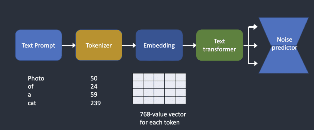
Below is an overview of how a text prompt is processed and fed into the noise predictor. Tokenizer first converts each word in the prompt to a number called a token. Each token is then converted to a 768-value vector called embedding. (Yes, this is the same embedding you used in AUTOMATIC1111) The embeddings are then processed by the text transformer and are ready to be consumed by the noise predictor.

Now let’s look closer into each part. You can skip to the next section if the above high-level overview is good enough for you.

Check tokens and embeddings of any prompt with this notebook.

Tokenizer

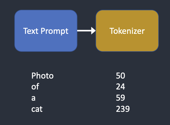
The text prompt is first tokenized by a CLIP tokenizer. CLIP is a deep learning model developed by Open AI to produce text descriptions of any images. Stable Diffusion v1 uses CLIP’s tokenizer.

Tokenization is the computer’s way of understanding words. We humans can read words, but computers can only read numbers. That’s why words in a text prompt are first converted to numbers.

A tokenizer can only tokenize words it has seen during training. For example, there are “dream” and “beach” in the CLIP model but not “dreambeach”. Tokenizer would break up the word “dreambeach” into two tokens “dream” and “beach”. So one word does not always mean one token!

Another fine print is the space character is also part of a token. In the above case, the phrase “dream beach” produces two tokens “dream” and “[space]beach”. These tokens are not the same as that produced by “dreambeach” which is “dream” and “beach” (without space before beach).

Stable Diffusion model is limited to using 75 tokens in a prompt. (Now you know it is not the same as 75 words!)

Embedding

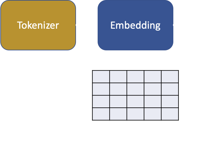
Stable diffusion v1 uses Open AI’s ViT-L/14 Clip model. Embedding is a 768-value vector. Each token has its own unique embedding vector. Embedding is fixed by the CLIP model, which is learned during training.

Why do we need embedding? It’s because some words are closely related to each other. We want to take advantage of this information. For example, the embeddings of man, gentleman, and guy are nearly identical because they can be used interchangeably. Monet, Manet, and Degas all painted in impressionist styles but in different ways. The names have close but not identical embeddings.

This is the same embedding we discussed for triggering a style with a keyword. Embeddings can do magic. Scientists have shown that finding the proper embeddings can trigger arbitrary objects and styles, a fine-tuning technique called textual inversion.

Feeding embeddings to noise predictor

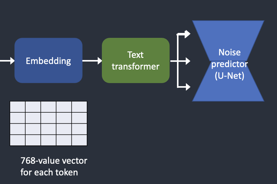
The embedding needs to be further processed by the text transformer before feeding into the noise predictor. The transformer is like a universal adapter for conditioning. In this case, its input is text embedding vectors, but it could as well be something else like class labels, images, and depth maps. The transformer not only further processes the data but also provides a mechanism to include different conditioning modalities.

Cross-attention

The output of the text transformer is used multiple times by the noise predictor throughout the U-Net. The U-Net consumes it by a cross-attention mechanism. That’s where the prompt meets the image.

Let’s use the prompt “A man with blue eyes” as an example. Stable Diffusion pairs the two words “blue” and “eyes” together (self-attention within the prompt) so that it generates a man with blue eyes but not a man with a blue shirt. It then uses this information to steer the reverse diffuse towards images containing blue eyes. (cross-attention between the prompt and the image)

A side note: Hypernetwork, a technique to fine-tune Stable Diffusion models, hijacks the cross-attention network to insert styles. LoRA models modify the weights of the cross-attention module to change styles. The fact that modifying this module alone can fine-tune a Stabe Diffusion model tells you how important this module is.

Other conditionings

The text prompt is not the only way a Stable Diffusion model can be conditioned.

Both a text prompt and a depth image are used to condition the depth-to-image model.

ControlNet conditions the noise predictor with detected outlines, human poses, etc, and achieves excellent controls over image generations.

Stable Diffusion step-by-step

Now you know all the inner mechanics of Stable Diffusion, let’s go through some examples of what happens under the hood.

Text-to-image

In text-to-image, you give Stable Diffusion a text prompt, and it returns an image.

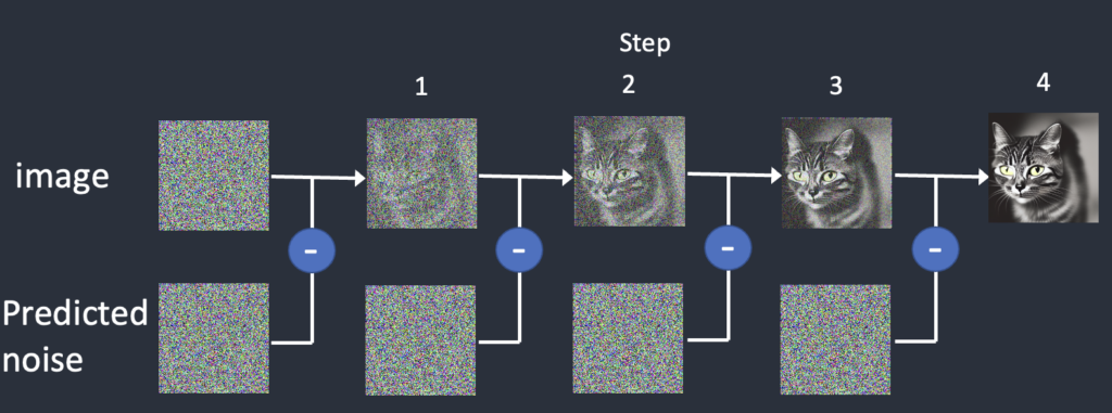
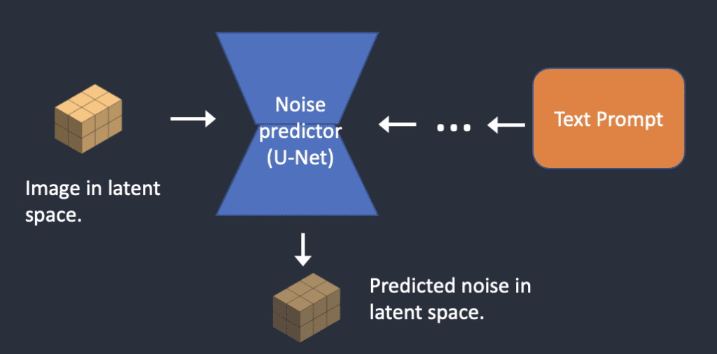
Step 1. Stable Diffusion generates a random tensor in the latent space. You control this tensor by setting the seed of the random number generator. If you set the seed to a certain value, you will always get the same random tensor. This is your image in latent space. But it is all noise for now.

Step 2. The noise predictor U-Net takes the latent noisy image and text prompt as input and predicts the noise, also in latent space (a 4x64x64 tensor).

Step 3. Subtract the latent noise from the latent image. This becomes your new latent image.

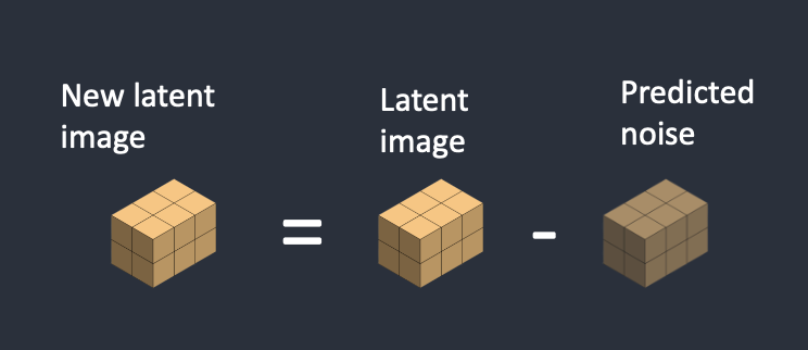
Steps 2 and 3 are repeated for a certain number of sampling steps, for example, 20 times.

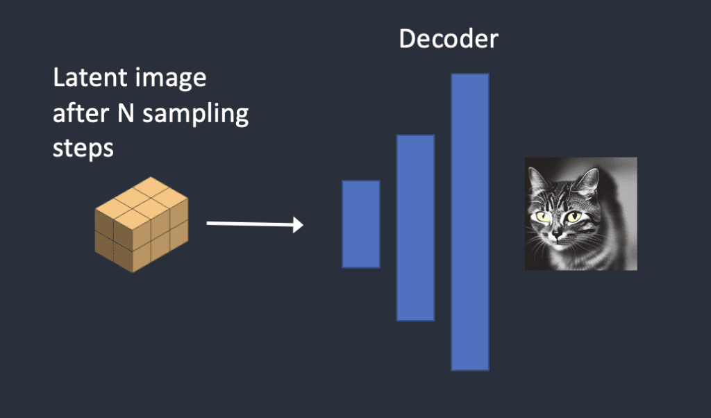
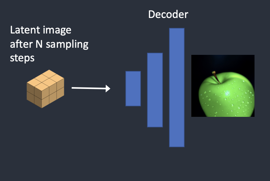
Step 4. Finally, the decoder of VAE converts the latent image back to pixel space. This is the image you get after running Stable Diffusion.

Here’s how the image evolves in each sampling step.

Noise schedule

The image changes from noisy to clean. Do you wonder if the noise predictor not working well in the initial steps? Actually, this is only partly true. The real reason is we try to get to an expected noise at each sampling step. This is called the noise schedule. Below is an example.

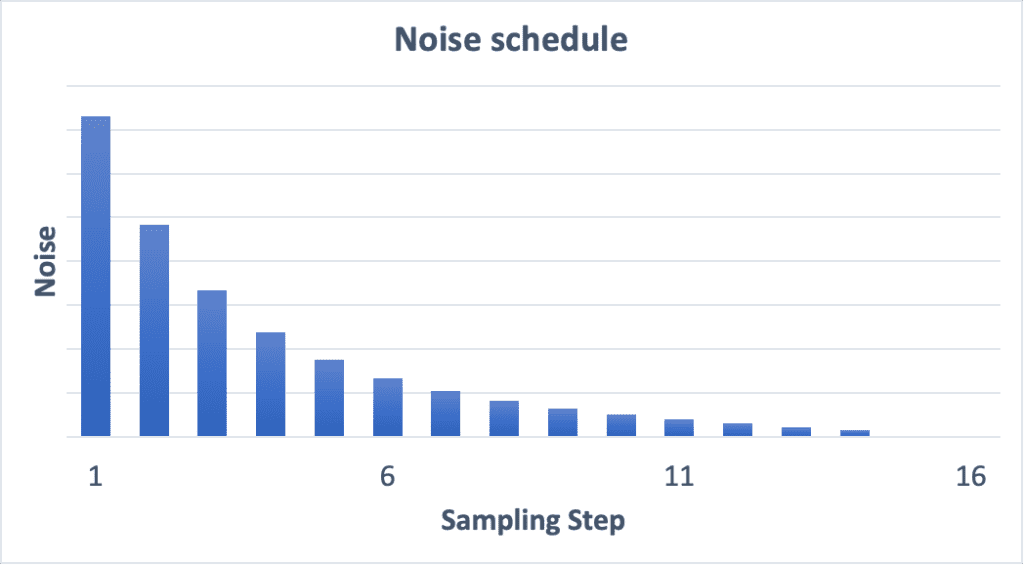
The noise schedule is something we define. We can choose to subtract the same amount of noise at each step. Or we can subtract more in the beginning, like above. The sampler subtracts just enough noise in each step to reach the expected noise in the next step. That’s what you see in the step-by-step image.

Image-to-image

Image-to-image transforms an image into another one using Stable Diffusion. It is first proposed in the SDEdit method. SDEdit can be applied to any diffusion model. So we have image-to-image for Stable Diffusion (a latent diffusion model).

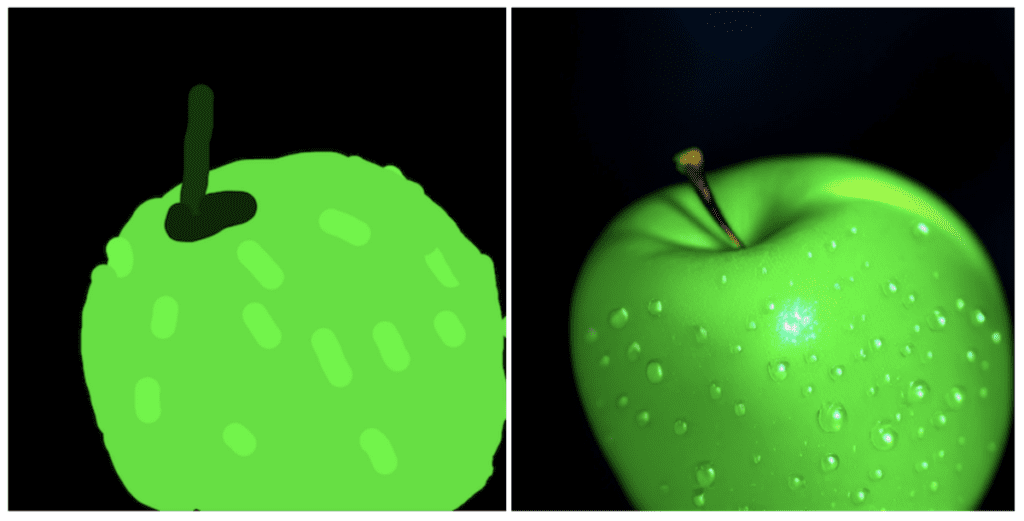
An input image and a text prompt are supplied as the input in image-to-image. The generated image will be conditioned by both the input image and text prompt. for example, using this amateur drawing and the prompt “photo of perfect green apple with stem, water droplets, dramatic lighting” as inputs, image-to-image can turn it into a professional drawing:

Now here’s the step-by-step process.

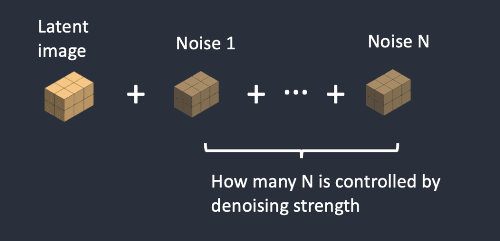
Step 1. The input image is encoded to latent space.

Step 2. Noise is added to the latent image. Denoising strength controls how much noise is added. If it is 0, no noise is added. If it is 1, the maximum amount of noise is added so that the latent image becomes a complete random tensor.

Step 3. The noise predictor U-Net takes the latent noisy image and text prompt as input and predicts the noise in latent space (a 4x64x64 tensor).

Step 4. Subtract the latent noise from the latent image. This becomes your new latent image.

Steps 3 and 4 are repeated for a certain number of sampling steps, for example, 20 times.

Step 5. Finally, the decoder of VAE converts the latent image back to pixel space. This is the image you get after running image-to-image.

So now you know what image-to-image is: All it does is set the initial latent image with a bit of noise and input image. Setting denoising strength to 1 is equivalent to text-to-image because the initial latent image is entirely random.

Inpainting

Inpainting is really just a particular case of image-to-image. Noise is added to the parts of the image you wanted to inpaint. The amount of noise is similarly controlled by denoising strength.

Depth-to-image

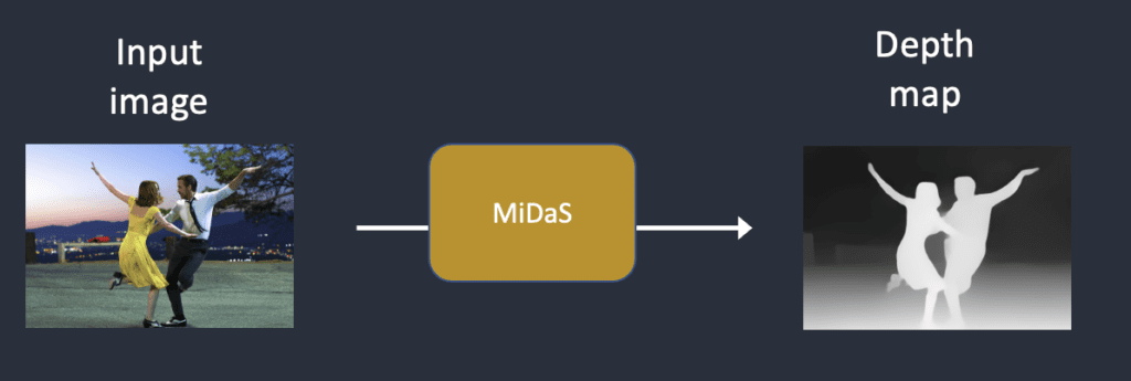
Depth-to-image is an enhancement to image-to-image; it generates new images with additional conditioning using a depth map.

Step 1. The input image is encoded into the latent state

Step 2. MiDaS (an AI depth model) estimates the depth map from the input image.

Step 3. Noise is added to the latent image. Denoising strength controls how much noise is added. If the denoising strength is 0, no noise is added. If the denoising strength is 1, the maximum noise is added so that the latent image becomes a random tensor.

Step 4. The noise predictor estimates the noise of the latent space, conditioned by the text prompt and the depth map.

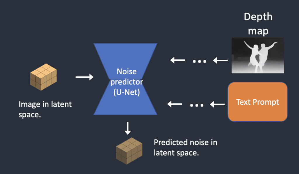
Step 5. Subtract the latent noise from the latent image. This becomes your new latent image.

Steps 4 and 5 are repeated for the number of sampling steps.

Step 6. The decoder of VAE decodes the latent image. Now, you get the final image from depth-to-image.

What is CFG value?

This write-up won’t be complete without explaining Classifier-Free Guidance (CFG), a value AI artists tinker with every day. To understand what it is, we will need to first touch on its predecessor, classifier guidance…

Classifier guidance

Classifier guidance is a way to incorporate image labels in diffusion models. You can use a label to guide the diffusion process. For example, the label “cat” steers the reverse diffusion process to generate photos of cats.

The classifier guidance scale is a parameter for controlling how closely should the diffusion process follow the label.

Below is an example I stole from this paper. Suppose there are 3 groups of images with labels “cat”, “dog”, and “human”. If the diffusion is unguided, the model will draw samples from each group’s total population, but sometimes it may draw images that could fit two labels, e.g. a boy petting a dog.

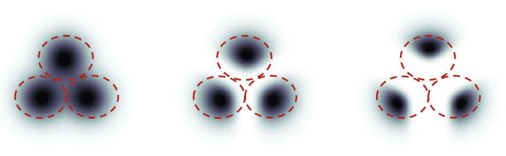
With high classifier guidance, the images produced by the diffusion model would be biased toward the extreme or unambiguous examples. If you ask the model for a cat, it will return an image that is unambiguously a cat and nothing else.

The classifier guidance scale controls how closely the guidance is followed. In the figure above, the sampling on the right has a higher classifier guidance scale than the one in the middle. In practice, this scale value is simply the multiplier to the drift term toward the data with that label.

Classifier-free guidance

Although classifier guidance achieved record-breaking performance, it needs an extra model to provide that guidance. This has presented some difficulties in training.

Classifier-free guidance, in its authors’ terms, is a way to achieve “classifier guidance without a classifier”. Instead of using class labels and a separate model for guidance, they proposed to use image captions and train a conditional diffusion model, exactly like the one we discussed in text-to-image.

They put the classifier part as conditioning of the noise predictor U-Net, achieving the so-called “classifier-free” (i.e., without a separate image classifier) guidance in image generation.

The text prompt provides this guidance in text-to-image.

Classifier-free guidance scale

Now, we have a classifier-free diffusion process using conditioning. How do we control how much the AI-generated images should follow the guidance?

The classifier-free guidance scale (CFG scale) is a value that controls how much the text prompt steers the diffusion process. The AI image generation is unconditioned (i.e. the prompt is ignored) when the CFG scale is set to 0. A higher CFG scale steers the diffusion towards the prompt.

Stable Diffusion v1.5 vs v2

This is already a long post, but it won’t be complete without comparing the differences between the v1.5 and v2 models.

Model difference

Stable Diffusion v2 uses OpenClip for text embedding. Stable Diffusion v1 uses Open AI’s CLIP ViT-L/14 for text embedding. The reasons for this change are

• OpenClip is up to five times larger. A larger text encoder model improves image quality.
• Although Open AI’s CLIP models are open-source, the models were trained with proprietary data. Switching to the OpenClip model gives researchers more transparency in studying and optimizing the model. It is better for long-term development.

The v2 models come in two favors.

• The 512 version generates 512×512 images
• The 768 version generates 768×768 image

Training data difference

Stable Diffusion v1.4 is trained with

• 237k steps at resolution 256×256 on laion2B-en dataset.
• 194k steps at resolution 512×512 on laion-high-resolution.
• 225k steps at 512×512 on “laion-aesthetics v2 5+“, with a 10% dropping in text conditioning.

Stable Diffusion v2 is trained with

• 550k steps at the resolution 256x256 on a subset of LAION-5B filtered for explicit pornographic material, using the LAION-NSFW classifier with punsafe=0.1 and an aesthetic score >= 4.5. 
• 850k steps at the resolution 512x512 on the same dataset on images with resolution >= 512x512.
• 150k steps using a v-objective on the same dataset.
• Resumed for another 140k steps on 768x768 images.

Stable Diffusion v2.1 is fine-tuned on v2.0

• additional 55k steps on the same dataset (with punsafe=0.1)
• another 155k extra steps with punsafe=0.98

In essence, they turned off the NSFW filter in the last training steps.

Outcome difference

Users generally find it harder to use Stable Diffusion v2 to control styles and generate celebrities. Although Stability AI did not explicitly filter out artist and celebrity names, their effects are much weaker in v2. This is likely due to the difference in training data. Open AI’s proprietary data may have more artwork and celebrity photos. Their data is probably highly filtered so that everything and everyone looks fine and pretty.

The v2 and v2.1 models are not popular. People use the fine-tuned v1.5 and SDXL models exclusively.

SDXL model

The SDXL model is the official upgrade to the v1 and v2 models. The model is released as open-source software.

It is a much larger model. In the AI world, we can expect it to be better. The total number of parameters of the SDXL model is 6.6 billion, compared with 0.98 billion for the v1.5 model.

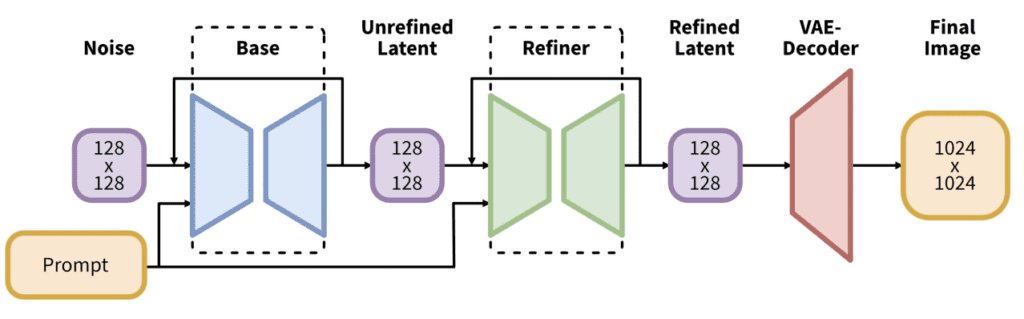
The SDXL model is, in practice, two models. You run the base model, followed by the refiner model. The base model sets the global composition. The refiner model adds finer details.

You can run the base model alone without the refiner.

The changes in the SDXL base model are:

• The text encoder combines the largest OpenClip model (ViT-G/14) and OpenAI’s proprietary CLIP ViT-L. It is a smart choice because it makes SDXL easy to prompt while remaining the powerful and trainable OpenClip.
•  New image size conditioning that aims to use training images smaller than 256×256. This significantly increases the training data by not discarding 39% of the images.
• The U-Net is three times larger than v1.5.
•  The default image size is 1024×1024. This is 4 times larger than the v1.5 model’s 512×512. (See image sizes to use with the SDXL model)

Ethical, moral and legal issues

Stable Diffusion, like other AI models, needs a lot of data for training. Its first version used images without copyright permissions. Though this might be okay for research, its commercial popularity drew attention from copyright owners and lawyers.

Three artists filed a class-action lawsuit against Stability AI, the commercial partner of Stable Diffusion, in January 2023. The next month, the image giant Getty filed another lawsuit against it.

The legal and moral issue is complicated. It questions whether a computer creating new works by imitating artist styles counts as copyright infringement.

Some interesting reads

• Stable Diffusion v1.4 press release
• Stable Diffusion v2 press release
• Stable Diffusion v2.1 press release
• Announcing SDXL 1.0 — Stability AI
• High-Resolution Image Synthesis with Latent Diffusion Models – research paper introducing Stable Diffusion
• The Illustrated Stable Diffusion – Some good details in model architecture
• Stable Diffusion 2 – Official model page
• Diffusion Models Beat GANs on Image Synthesis – Research paper introducing classifier guidance
• Classifier-Free Diffusion Guidance – Research paper introducing classifier-free guidance
• Deep Unsupervised Learning using Nonequilibrium Thermodynamics – Reverse diffusion process